Explanation of a self-learning, evolving neural network

In this article we’ll go through the application of a self-learning, evolution-based genetic algorithm that augments its own topology. Confused? I can imagine; those are some big words. Stay with me though, I promise you’ll see the beauty of this algorithm at the end of this article.

In order to understand neuro-evolution-algorithms as clearly as possible I’ve programmed a little game called Dots that will illustrate the way the algorithm works. I’m trying to describe what happens in lay-mans terms, not focusing on programming or math. The goal is that you understand the general working of neural networks and see their possibilities and applications.

The algorithm we’re using is called NEAT (NeuroEvolution of Augmenting Topologies) by Ken Stanley. After you’ve read this article you’ll have a rough understanding of how it works and what it’s benefits are. We’ll do this in the following steps:

1. Description and goal of the game
2. The dot; inputs and outputs
3. Evolving dots
4. Putting it all together — quick summary
5. Other applications

1. Setup and game goal

Go to mike-huls.github.io/neat_dots and press the big, green play button in the top right.

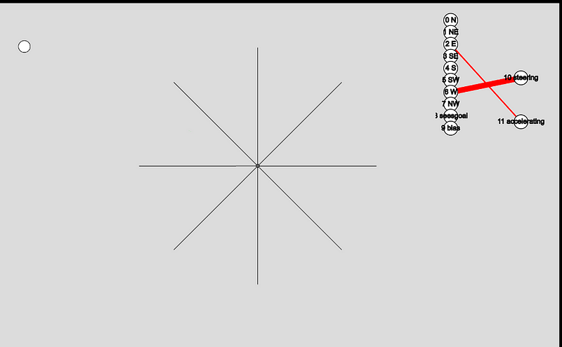
The first thing you’ll see is a bunch of circles spawning in the bottom right, after which they all move along like a drunk airplane pilot. These circles are called dots and they spawn by the hundreds. At the beginning of the game a few hundred dots spawn and start moving about. If they crash into a black border they die. The black border at the edges is an obstacle. If a dot touches one of these it dies. You can click the “add obstacle” button to draw new obstacles.

Once all dots are dead or after a certain time passed, a fresh new generation of dots spawn. The goal of each dot is to reach the goal in the upper left. The goal of the game is to evolve the dots in such a way that they reach their goal in the fastest, most optimized way. Let’s find out how this works!

2. Introducing our contestants

Play the game a few times, try some different obstacles and check out how the dots react. Now it’s time to get to know them a little better. First we’ll analyze the dot itself; how does it interpret the environment, what can it do and how does it decide to do this?

Actions, sensors and decision making

Dots can move in two ways: they can accelerate and decelerate and steer to the left and right. The dots goal is to accelerate and steer in such a way that it reaches the goal; the white circle in the top left.

But how does a dot decide when to accelerate or steer? That all depends on the surroundings of the dot. Each one has 9 sensors; it can look in 8 directions (represented by the lines in image 1). In addition it can detect whether or not it sees the goal. The bias-sensor is always set to 1; in case all other nodes are ‘off’.

All sensors have a value between 0 and 1. The closer it gets to an obstacle, the higher the value gets to 1. If no obstacle is detected the sensor is 0. The seesGoal sensor works a little different; it’s either 0 or 1.

Actions have a value between -1 and 1. A negative value will decelerate or steer to the left, a positive value will accelerate or steer to the right.

Connecting the dots; creating a brain

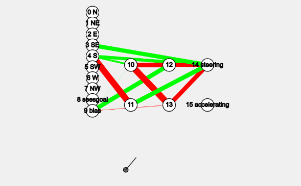
Our goal is to have the dot act upon its sensors; it interprets its environment in order to survive and touch the goal. The dot has to learn that it shouldn’t steer to the left if it detects an obstacle there. Each dot has a brain that makes it possible for a dot to do exactly this. Think of the brain as the way the sensors are connected to the actions. This is also called the neural networks’ topology (remember, from the name of the paper?). You’ll see the sensor-nodes in the first column and the action-nodes in the second.

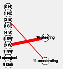
In the top-right of the game you see the brain of the most successful dot. You see a close-up in image 2. Since the game just started, this brain is fairly simple but it can be a lot more complex:

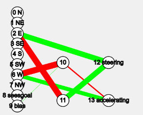
Not only has the dot created more connections, it also created some extra nodes. This way it can interpret multiple sensors at once. It can for example detect an obstacle in sensor 1 and 2, then combine this observation with an obstacle in sensor 0 and let the outcome of this influence steering.

Creating extra nodes and edges is pretty special; in most neural algorithms you’ll have to define your topology (brain) beforehand. It assumes you know which nodes need to be connected. The beauty of NEAT is that it starts off with the simplest topology; just inputs (sensor) and outputs (actions) and then builds its own topology. This guarantees a minimal network structure and is generally really cool. Later we’ll discuss how the algorithm evolves the topology.

In image 2 we see that sensor 6 is connected to steering with a thick red line. Red indicates that the connection is negative. The thickness indicates that the weight of the connection is high; sensor6 has a large, negative influence on steering. In other words: when the dot detects something to its left it steers to the left, right into the obstacle. This is a bit dumb but its okay, our little dot is still learning.

3. Evolving dots

The beauty about the neural network we’re using is that we haven’t defined anything up front. The dot is not programmed to steer away from the wall, nor has it even the slightest idea that walls are so deadly. The dot is, however, programmed to learn. In this section we’re going to dive in how the dot is learning, how it shares its knowledge and how this knowledge is being passed over into next generations. The general order looks like this:

• calculate dot fitness
• speciate
• crossover
• mutate

Survival of the fittest

When a dot spawns there are not many connections between its sensors and actions. One random connection is created and is given a random weight, indicated by its thickness. In the image above, the dot will crash itself right in to the wall. The dot has no idea whether this is going to be a good decision for him; it has no idea whether it’s doing the right thing. In order to learn it has to have some kind of measure of what is good for him. This is where fitness comes in.

You might recognize this term from Darwin. Fitness says something about how well you’re adjusted to your surroundings. Think of it as a dog receiving a treat if it does something good; we’re reinforcing ‘good’ behavior. In the game we can see the fitness for the best performing dot in the Model information segment.

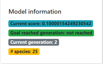
We define in the code when a dot is doing well. In this particular example I’ve defined fitness as follows:

• If the dot hasn’t seen the goal yet it needs to go in exploration mode: fitness is 0 to start with and increases the more distance it covers.
• If the dot has seen the goal it means that the dot has been in a position from where it can reach the dot. First the dot receives a bonus for this; then its fitness is defined by the distance it dies from the goal; shorter is better
• If the dot has reached the goal it receives a bonus once more. Fitness is then defined by the shortest amount of steps it needs to reach the goal; ensuring that we get there as fast as possible.

Great! We have codified when a dot performs well. With this information we can execute on of the most important parts of this algorithm: speciation.

Speciation

Now that we have a way to compare dots we can reveal why we spawn hundreds of them at the same time: they’re going to experiment, share knowledge and evolve. This is how it works: after each of the dots has done its thing; racing around, optionally crashing into walls, it’s time to see who’s best. First we’re going to compare all the dots based on their brain. Dots that are pretty alike are going to be grouped into a species.

You can recognize species in the game; sometimes you’ll clearly see one group of dots doing quite something else from the rest. Maybe the take the north-bound route while another group goes south around the obstacle. This is because their brains are significantly different.

We’ll order dots within each species based on their fitness and then kill the bottom half of each species. This may sound a bit cruel and you’d be completely right. But just like in nature; only the fittest survive. Also notice that dots only have to compete within their species; this is to protect innovation. Newly evolved dots might not perform all that well at first and need a few generation to really get going. It would be sad if they’d go extinct before reaching their true potential.

Lastly it’s time to kill off stale species. We can detect this by examining the fitness score of the best performing dot within the species. If it hasn’t improved for a few generations it’s become stale and it’s time to go.

Crossover

We’ve killed a lot of bad dots in the last few paragraphs. Let’s re-populate by taking our best dots and breed ‘m to pass along those good brains. Within each species pairs of random parents are selected. Dots with a higher fitness score have a higher change to be selected. Each pair will combine their best traits in creating a child. The brain of their offspring will be a combination of their parents brain. After this step our population will be of the same size as in the beginning of the generation.

Mutate

The last step, before a new generation will start, is mutation. In order to keep innovation going every dots brain is randomly mutated. This means that each dot gets either a new node or a new connection.

This step introduces some randomness in all of the dots. In some cases this will be beneficial, other dots will suffer from their new brains. Thankfully, thanks to speciation, the dot will have some time to ‘tune’ its brain.

Do it again

Our new generation is ready for a next round. All dots will spawn again, hopefully navigate with a little more success and eventually reach the goal or die. Then their fitness is calculated again, all dots are speciated, culled, bred and mutated and we’re ready for the next cycle. Each generation will be a bit better than the previous and eventually the goal will be reached.

4. Putting it all together

I think NEAT is pretty special because it requires you to define so few things beforehand. In many statistical techniques there are many requirements. In many genetic algorithms we need to define our topology (the dots brain) beforehand. NEAT starts out with a minimal topology, just connecting the inputs and outputs, and then slowly adds complexity to keep it as simple as possible. In addition it protects innovation through using species; dots only have to compete within their species. In addition it breeds the best-performing dots, combining the best traits of both parents.

The downside, compared to other statistical techniques, is that the model that NEAT produces is quite complex. Where we can extract a simple formula when using linear regression, a brain in NEAT can be extremely complex and hard to grasp in a simple formula. Where we can use linear regression to determine whether or not there is a linear relationship between variables, the relationship in NEAT can be hard to see.

5. Other applications

In the case of dots we connect dot-sensors to some actions it can perform. This doesn’t have much real-world value but thankfully NEAT isn’t limited to navigating clumsy circle’s through an obstacle maze. In this section we’ll examine a hypothetical example of how we can apply NEAT in the real world.

Determining house prices

You have a dataset that contains house characteristics and the selling price. We’ll apply NEAT to create a brain that can most accurately determine the selling price based on the characteristics.

A dot has 9 sensors: sight in 8 directions and whether it can see the goal. As an example our house price-brain will have house-surface, land-surface, number of bedrooms, building year, has driveway and number of parking places. W have to scale all of these values between 0 and 1 where 0 is the minimum building year and 1 is the maximum, for example. Our output will be the house price. The house price will also be a number between 0 and 1; it’s mapped between the minimum and maximum house prices in our training data.

Just like we spawned a few hundred dots, now we’ll spawn a few hundred “house-brains” and give all of them a few records of data from our training set. The data flows through the brain to calculate the house price. We’ll compare this with the actual house price. The difference is the fitness; smaller is better. Then the NEAT algorithm kicks in again. The brains are scored, sorted, culled, speciated, bred and mutated, after which we’ll feed them data again.

The brains will change their topology and adjust their weights. After many iterations we can take the best-performing brain and feed it some new data in order to predict the house price.

Conclusion

When I first read the NEAT paper I fell in love with the algorithm because it closely resembles nature. We’re talking about species, fitness, genomes, crossover, parents and offspring. To me it was fascinating that we can program such natural behavior. I really liked this algorithm for its flexibility, elegance and efficiency.

I hope this article served as an introduction to this great algorithm and that it was clear enough to show you the beauty of it. If you have suggestions/clarifications please comment so I can improve this article. In the meantime, check out my other articles on all kinds of programming-related topics. Happy coding!

— Mike

P.S: Like what I’m doing? Follow me!